Spatial analysis for infectious disease epidemiology using R: Part 2
As a reminder last time we covered going from the data to a visually appealing choropleth map. My qualitative interpretation of this map led me to believe there is a non-random distribution of infections in the neonatal ICU. Your interpretation may differ from mine, hence the need some statistical testing.
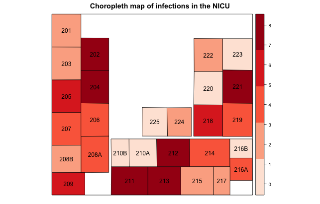
In this post we answer the two overarching questions from last time: 1) are the infections distributed in some non-random fashion in the unit, and 2) does proximity to an infection influence one's own risk? These questions can be answered using multilevel techniques to assess non-randomness and spatial techniques to detect autocorrelation among neighbors.
Assessing randomness
The easiest test to perform is a global test of whether the proportion of outcomes (i.e., infections) are equivalent across all 28 beds. Let's say there were 100 infections total. If there was random distribution we would expect approximately 3 infections per bed over time. This can be tested using a simple prop.test, as detailed elsewhere on this blog.
A better way to do this test is to construct an empty multilevel regression model, where our only predictor is the clustering unit. Since we're returning to individual level data (long format) at this point, our outcome is binary: either an infection occurred for that patient during their stay, or it did not. Thus we'll need a generalized linear mixed effects modeling approach, such as implemented in the lme4 package.
A simple empty model looks like:
model = glmer(Infection ~ (1 | Bed), family=binomial(), data=NICU)
where Infection is the binary outcome, bed is the clustering unit, and NICU is the long format data frame. Occasionally the glmer algorithm fails to converge, which, after you've checked the usual suspects, is likely a false positive. To circumvent this occurrence, one can use a different optimizer, e.g.:
model = glmer(Infection ~ (1 | Bed), family=binomial(), data=NICU , control=glmerControl(optimizer="bobyqa"))
model = glmer(Infection ~ (1 | Bed), family=binomial(), data=NICU , control=glmerControl(optimizer="nloptwrap"))
Turning to the summary(model) output, we can either estimate the global variance, getME(model, "theta") useful for computing the median odds ratio, or see if there is non-random distribution by examining the fixed effect of the intercepts. A significant intercept indicates significant clustering, or non-random distribution. Also at this point, we can introduce additional individual or group level covariates into the model to try to isolate the independent predictors of infections. More detail has been provided elsewhere on this blog.
As my model has significant clustering, we turn attention to the final part of exploratory analysis: spatial autocorrelation.
Neighbor influences
The first step in the spatial analysis is to define what a neighbor means by using the function poly2nb in the spatial dependence package. This could be based on contiguity of geographic boundaries, distance between their centroids, or some other parameterization. R includes algorithms for detecting contiguity or distance:
sa.nb = poly2nb(NICU_map, queen=T, snap=10)
This function creates a neighbor list for the NICU_map shapefile data by contiguity (queen=T) or a distance less than or equal to 10 units (snap=10) between shapefile features. The exact unit your map uses has been determined by the coordinate reference system, explained in more detail here.
After running this function, you can double check the neighbors are defined appropriately by plotting the output, for a reasonable number of neighbors as I have for this project. First we plot the shapefile itself, then we plot the neighbor list as red lines.
plot(NICU_map)
plot(sa.nb, coordinates(NICU_map), add=T, col="red")
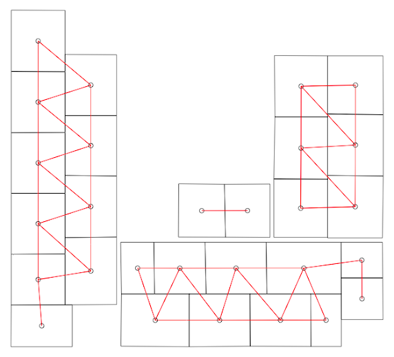
Unfortunately the algorithm did not quite succeed. I need to define a slightly different set of neighbors based upon expert opinion on infectious disease transmission with this NICU. I can readily accomplish through code similar to this: sa.nb[[12]] = as.integer(c(sa.nb[[12]], 18)) To break this down, after creating the neighborlist object with poly2nb, I am accessing the 12th feature in the shapefile and telling R that in addition to the existing neighbor list, shapefile feature #18 should also be considered a neighbor. Likewise I need to reciprocate this modification with the 18th feature as follows: sa.nb[[18]] = as.integer(c(sa.nb[[18]], 12)) How do I know which feature corresponds to which bed? By simply outputting the feature list which has the bed attributes: NICU_map@data. This can become fairly tedious but is nonetheless necessary if the poly2nb algorithm did not otherwise define the neighbors correctly.
With the neighboring list correctly defined, we can apply a test for spatial autocorrelation, for example Moran's I. We can use Moran's I to test for spatial autocorrelation from either the crude number of infections per bed or from the adjusted measure using the random intercepts from the generalized linear mixed model.
To do either test, we first need to create a representation of the binary weights from the neighborlist with the following command:
sa.wt = nb2listw(neighbours=sa.nb, style="B")
Now we can perform a crude test for autocorrelation using Moran's I as follows:
moran.mc(NICU_map$Infections, listw=sa.wt, nsim=1000)
Alternatively if there is strong confounding suspected, we can use the adjusted random intercepts from the mixed model to test for autocorrelation:
moran.mc(ranef(model)[[1]][[1]], listw=sa.wt, nsim=1000)
More information about this approach can be found on page 15 in the R vignette entitled: CARBayes version 4.6: An R Package for Spatial Areal Unit Modelling with Conditional Autoregressive Priors.
Two additional notes for consideration. First, if you have geographic features with zero outcomes occurring, you may need to add the argument zero.policy=T in the poly2nb and nb2listw functions to allow for zero length vectors. Second, using the mixed model approach to Moran's I but specifying an empty model should yield similar results to the crude test described above.
The output from Moran's I will be the statistic itself and a p-value indicating whether spatial autocorrelation was detected. If there was autocorrelation, a spatial correlogram is a useful tool to assess where the correlations are coming from.
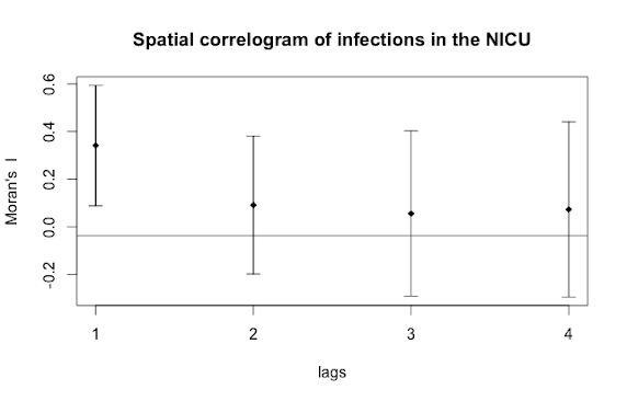
Here we can see that the immediate neighbor (lags=1) is influencing an individual's risk of infection, both the neighbor's neighbor (lags=2) and neighbor's neighbor's neighbor (lags=3), and so on, are unremarkable. Finally, we can conduct a spatial type of regression analysis known as a spatial lag model that accounts not only for the correlation by spatial unit but the autocorrelation, if present. But that's a topic for a different day and this concludes this two-part post on exploratory spatial analytic techniques useful for infectious disease epidemiology.
For additional information here are some example epidemiological studies that utilize spatial methods:
- Geospatial patterns in human papillomavirus vaccination uptake: evidence from uninsured and publicly insured children in North Carolina.
- The built environment and depressive symptoms among urban youth: A spatial regression study.
- Ecological factors associated with pandemic influenza A (H1N1) hospitalization rates in California, USA: a geospatial analysis.
Cite: Goldstein ND. Spatial analysis for infectious disease epidemiology using R: Part 2. Feb 4, 2017. DOI: 10.17918/goldsteinepi.