Neal D. Goldstein, PhD, MBI

Notes on causal inference in observational epidemiology

I don't do a lot of causal inference methods work. I view myself as somewhat of an outsider to this core area of epidemiology. Although I always bring a well specified conceptual model to my analyses, I have infrequently invoked some of the more sophisticated approaches to causal inference that I learned about in school, heard presentations at conferences (often SER), or (most often) have read about in epidemiology journals. This blog post is my attempt to come back up to speed with the field by crudely cataloging the methods used in observational epidemiology; not so much to be an expert in these approaches, but rather to enumerate some of the more common and current approaches for an understanding of when these techniques should be invoked. This cataloging process will start with the highest philosophical level, and then proceed to the applied epidemiology level. My line of inquiry is heavily indebted to a wonderful article critiquing the de facto counterfactual approach to causal training among epidemiologists that got me thinking along these lines.

It is important to note at the outset that when epidemiologists talk about causal inference there are two senses to the concept: the philosophical sense and the technical sense. The philosophical sense is a "set of convictions about how epidemiologists should think about causality" while the technical sense "concerns a collection of mathematical tools and methods" (Vanderbroucke et al. 2016, IJE). The methods that I introduce later are not a focus of any particular causal camp; although they may arise out of a specific philosophical approach, they can be viewed as a distinct entity. In fact, this is how epidemiological training often proceeds. Trainees typically take a course on causal inference that is weighted towards the philosophical aspects of the concept, while the tools and techniques to achieve causal inference are taught in advanced epidemiological methods courses. As an aside, causal inference should not to be conflated with statistical inference as these are distinct concepts. Thus, we can summarize by stating that the theory of causation is firmly grounded in philosophy, while the tools for causal inference arise from modeling causation.

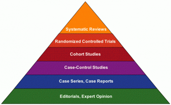
Students of philosophy will recognize that there are many different schools of thought with respect to causal thinking. Philosophical causality includes theories of regularity, probabilism, causal processes, interventionism, and, of course, counterfactualism, to name but a few. Counterfactualism has more or less become the de facto school of thought for epidemiology: what would have happened had the exposure been different? It is, of course, impossible in reality to answer this question. Thus we rely upon study designs that attempt to recreate the counterfactual condition between exposure groups. In the idealized setting nothing else differs between individuals except the exposure, and if causally related, the eventual outcome. This is also discussed in methodological language as the potential outcome approach: what is the potential outcome by varying treatment assignment? At this point, some purists including Vanderbroucke draw a distinction between the potential outcomes approach and philosophical counterfactualism, and argue that potential outcomes is in fact an interventionist approach to causal thinking. The interventionist approach to epidemiology suggests that for a public health question to be addressable through causal methods, we must be able to intervene on the exposure. Whether this distinction is important for the applied epidemiologist, I will leave that up to the reader. An intervention is the essence of the randomized controlled trial (RCT), and as we are taught in school, the RCT is atop the pyramid of evidence of causality.

In observational epidemiology, the paradigm has become how to best mimic the RCT through proper study design and analysis, essentially replicating the unbiased exposure assignment inherent in the RCT. Vanderbrouke elegantly argues why this restricted mindset is damaging to our field. For example, interventions are rarely well-specified, may be inconsequential to specify, and can change over time because what is not intervenable today may very well be tomorrow. Further, some interventions are impossible; one cannot intervene upon age, race, or other immutable characteristics which are linked to health-related outcomes, such as through discrimination. Regardless of whether one labels our approach interventionism, counterfactualism, or some other philosophical construct, the methods used in epidemiology are described in terms of potential outcomes framework largely due to the work of Donald Rubin and the Rubin Causal Model, so I will proceed using this language.

In order to compare the potential outcomes, epidemiologists strive to create the counterfactual condition. We cannot estimate the causal effect for an individual (because the counterfactual does not exist nor are we necessarily interested in the individual effect), so we estimate average causal effects. The unobserved outcome can be thought of as a missing data problem. The counterfactual condition can be achieved through exchangeability of the exposure groups (randomizing the exposure, when possible), mendelian randomization and instrumental variables (see Sheehan et al. 2008), difference-in-difference approach (origins in econometrics, when exchangeability in exposed and unexposed groups cannot be assumed), and so on. For the observational epidemiologist, the exchangeability criteria is paramount: how do we ensure that when the exposure groups are not randomized in the true sense of the word, we have selected, measured, and analyzed a study population as if they were? And this assumes that we have, in fact, a study population available to us. What if the exposure/treatment/intervention was hypothetical or planned for the future? Observed data may not exist. Our methods then become one of speculation. Suppose a person had received treatment, what would have happened? The potential outcomes are the outcomes that could be observed for each unit under the different exposure conditions.

Let's turn our attention to methods for causal inference used in epidemiology to answer the question, Does X --> Y? In the most simplistic case, let's assume there is no confounding or missing data, X and Y are correctly measured, there is a consistent linear relationship between the two variables, and Y does not cause X (no reverse causality). If this were the case – along with other assumptions omitted here – then we could fit a simple regression model and, if we see a statistical association, infer a causal one. Yet clearly these bold assertions cannot be guaranteed in observational, or for that matter, even experimental epidemiology. Therefore we need to turn to more sophisticated methods that can deal with a host of such methodological challenges. I've attempted to categorize these below. This list is not meant to be exhaustive, nor mutually exclusive (one may employ multiple methods), but is a starting point for considering the causal approach to take. Also provided are links to some of the seminal papers in the area.

• Observed data methodology: observational data already exist or can be collected.
• Traditional regression with covariates informed from causal diagrams including DAGs. This is probably the most frequently undertaken type of analysis because of its simplicity yet it also carries the greatest number of assumptions that are not likely to be met. These methods may include analysis of case-control data (e.g., logistic regression), cohort data (e.g., Poisson or Cox regression), longitudinal data and multilevel data (e.g., mixed-effects regression), and so on.
• Methods for improved control of confounding, covariate balancing, and reduced model dependency.
• G-computation. Estimating parameters had the observational study been a perfectly randomized experimental study. (see Robins 1986)
• Propensity (exposure) scoring and doubly robust estimation through propensity score matching and multivariable regression. The propensity score estimates the probability of exposure to mitigate the dimensionality of multiple potential confounders.(see Rosenbaum and Rubin 1983).
• Time-varying effects of exposures or confounders. The exposure (or covariates) may be influenced by covariates (or exposure) or the outcome over time. A nice overview of these methods is provider by Daniel et al.
• Structural nested models fit via G-estimation (see Robins et al. 1992).
• Marginal structural models fit via inverse probability weighting (see Robins et al. 2000).
• Decomposing exposure to outcome effects in the context of endogenous variables. I've previously written about these approaches on this blog.
• Structural equation modeling and traditional mediation analysis, such as Baron and Kenny effect decomposition or Sobel product of coefficients, with a variety of extensions.
• Counterfactual approach. Simulation-based approach to mediation analysis, similar to G-computation.
• Negative controls. I include negative controls here as an example of a design strategy that eschews exchangeability between groups to have a comparison group that differs in an important way to detect possible biases (see Lipsitch et al. 2010).
• Unobserved and synthetic data methodology: observational data do not exist nor can be collected at the present time.
• Observed data methodology can be applied over a synthetic data set or existing data set but with missing outcomes, for example, G-computation to predict outcomes scaling up an existing intervention.
• Systems modeling approaches. The confusion over the terminology here makes categorization different. See this article for a discussion of these approaches in causal inference.
• Agent-based models. This class of models simulate an exposure among individual agents to estimate the outcome effect. Sometimes called complex systems [dynamic] approaches.
• Dynamic transmission models. This class of models also simulations an exposure, yet operates at group levels, thus has fewer assumptions than agent-based models. Sometimes called system dynamic models.

Almost all of these methods have various extensions, such as dealing with case-control and survival (time-to-event) data, missing data, semi- and non-parametric approaches, as well as have a variety of assumptions that must be met. Sensitivity analyses are used throughout these methods to check for the robustness of assumptions and are a final step to guard against bias before inferring causality.

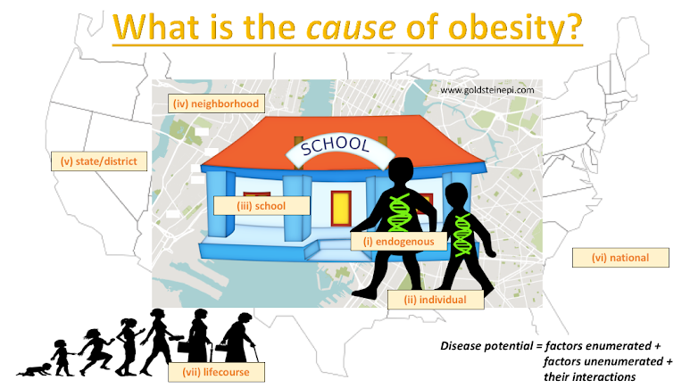
To conclude this post, I'd like to borrow an example from Sandro Galea: What is the cause of obesity? Among the myriad potential causes, the authors list:

"(i) endogenous factors such as genes and factors influencing their expression; (ii) individual-level factors such as behaviours (size of food portions, dietary habits, exercise, television-viewing patterns), education, income; (iii) neighbourhood-level factors such as availability of grocery stores, suitability of the walking environment, advertising of high caloric foods; (iv) school-level factors such as availability of high-caloric foods and beverages and health education; (v) district or state-level policies that regulate marketing of high caloric foods; (vi) national-level surplus food programmes, other food distribution programmes and support for various agricultural products; and (vii) from a lifecourse perspective history of breastfeeding, maternal health and parental obesity"

Here's what a pictorial representation of the cause of obesity may look like:

To paraphrase from the Galea article, the analytic methods of epidemiology struggle in the area of complex exposure patterns such as seen in chronic diseases like obesity. Exposure X is not necessarily ever a single variable and the epidemiologists usually makes strategic decisions as to what component of X to model. The decision could be based on convenience (available data), desired outcome (if making policy recommendations), or other pragmatic reasons. One could also model the upstream factors, and argue the other factors are mediators, but is it more difficult to intervene on the distal determinants. One could also attempt to fit a multilevel model, but given the many levels in this framework, the data will become too sparse too quickly. Both of these approaches also require observed data. A third possibility is to create a synthetic world that represents these factors and use systems modeling approaches to ascertain there independent contributions to the outcome. Regardless of the approach to modeling, a major implication of a complex relationship such as this is that there is no single view of causality (philosophical or technical) that is adequate. And in the end, I largely agree with the ideas of Vanderbroucke that our field should embrace causal pluralism and other non-counterfactual strategies that rule out alternative evidence, such as triangulation of evidence and negative controls (see Howe et al. 2012 for an example). I would further add to this we should also revisit (abandon?) the hierarchy of evidence as that enforces the RCT as the be-all-end-all study design. As the philosophers have known for centuries, there are multiple valid views of causation, and it is counterproductive and even detrimental to epidemiology to get restricted to only counterfactual or interventional theories. Rather we should embrace the diversity of approaches and theories to answering the most fundamental question, How can we improve the public's health?

Cite: Goldstein ND. Notes on causal inference in observational epidemiology. Feb 11, 2019. DOI: 10.17918/goldsteinepi.