Epi Vignettes: Interaction and effect modification
A brief synopsis of epidemiologic study design and methods with sample analytic code in R.
Returning to the Epi Vignettes series I've been writing, this post focuses on the concepts of interaction and effect modification. These concepts are generally introduced in an intermediate level epidemiology course and for the most part are treated synonymously in their interpretation, with the difference being how they are assessed. I was trained that effect modification is assessed via stratification on a third variable, while interaction is assess via a product term in a regression model.
While this simplification may be acceptable under most circumstances, there are some subtleties to assessing interaction and effect modification that I recently appreciated after peer review from several manuscripts. The terms in fact should not be used synonymously, as VanderWeele noted, and there is an important distinction. Although this distinction can be demonstrated statistically (as done in preceding article), I find a pragmatic definition more important. For the rest of this post, assume X and M are two exposures of interest, and Y is the outcome. The parameterization of the variables is unimportant as this time. Essentially we can say that effect modification (sometimes called effect heterogeneity, or heterogeneity of effects) occurs when, as a researcher, we have the ability to intervene on only one exposure (X), and interaction (sometimes called joint effects) occurs when we have the ability to intervene on both exposures (X and M).
Let's take two examples. Example 1. We are interested in assessing the relationship between race (X), drug use (M), and HIV status (Y). Since we cannot "intervene" on race, but only drug use, an effect modification approach is appropriate. Example 2. We are interested in assessing the relationship between alcohol use (X), drug use (M), and HIV status (Y). Since we can intervene on both alcohol and drug use, an interaction approach is appropriate. Of importance, these are causal definitions; statistically both effect modification and interaction may be assessed with an X*M product term in a regression model.
Approaches to testing for effect modification/heterogeneity of effects include stratified tests (e.g., Breslow-Day, Wald) or regression-based tests of interaction. For an excellent review of effect heterogeneity, see this article by Kaufman and MacLehose. Of note, the authors caution not to overly rely on the p-value of these tests as they may be underpowered to detect a difference thus concluding effect homogeneity, but rather compare the magnitude of effects within the strata of variable M. Generally stratum-specific estimates are used in the case of effect modification, especially when M is binary or has a relatively few number of categories. Otherwise the methods become unwieldy.
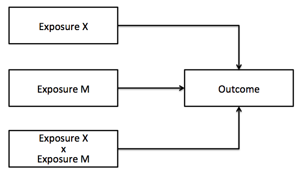
As most researchers seem to prefer a regression based approach to testing for interaction the rest of this blog post will assume a product term (X*M) in a regression model, yet assessing interaction is more than a product term in a regression model: there is statistical interaction (literally the result of the statistical test for the interaction term) and causal interaction (whether intervening on the variables X and/or M will have a causal effect on outcome Y). For now, X*M will be treated as a statistical interaction.
Depending upon the type of regression, the statistical interaction may be additive, multiplicative, or both. Additive interaction stipulates the summed effect of X and M will be greater than their individual effects, while multiplicative interaction stipulates that the product of X and M will be greater than their individual effects. As may be inferred in a straight linear regression model, which is on the linear scale, the interaction term represents additive interaction. In a generalized linear regression model such as logistic or Poisson regression, which is on the log scale, the interaction term represents multiplicative interaction. Stated another way, the multiplicative scale is a comparison of relative measures of association across strata (relative risk/odds ratio), while the additive scale is a comparison of difference measures of association across strata (e.g., attributable risk/risk difference). As absolute measures are more frequently used in in public health practice to demonstrate how interventions affect an outcome, it may be preferable to report additive interactions. However, since the X*M term in generalized linear regressions only indicate multiplicative interaction, the additive component must be manually calculated, and depends in part on the parameterization of X and M:
- If X and M are binary, the relative excess risk due to interaction (RERI; more recently referred to as the interaction contrast ratio) is a commonly used measure that is readily calculated. See Richardson and Kaufman for the methods of calculating RERI and its precision.
- Knol et al. discuss the implications of calculating RERI when either X or M are continuous. Interactions with continuous variables should be mean centered as needed.
- While RERI is commonly used, there are additional measures of additive interaction including the attributable proportion due to interaction (AP) and the synergy index (S). Knol et al. provide a nice overview and calculator for these measures.
- In fact, Skrondal advocates for use of the synergy index as he demonstrated that when the regression models include potential confounders (as in the majority of cases) RERI and AP may be biased measures of additive interaction, while S was unbiased.
- One additional caveat, as discussed by Knol et al., the methods for additive interaction are all derived from the case where X and M's effect on Y is risk-based. That is the ratio measure >1.0. In the case where X and M's effect on Y is protective (ratio measure <1.0), the variables need to be re-parameterized to risk factors. For categorical measures, this means changing the reference group to the one with the lowest risk, thus all other groups convey excess risk. This should be done for all variables as warranted in the same model (not one at a time). In the presence of a continuous measure, advice was not given, however one approach may be to subtract the measure from the lowest risk group. For example, consider gestational age for the infant where infants of longer gestations will have fewer morbidities and mortality, thus each unit increase in gestation is protective. To make this a risk-based measure, one can subtract gestation from 40 (corresponding to the average gestation), thus each unit increase in gestation corresponds to the offset from 40 and is thus a risk.
- In all cases, the preferred method for reporting the precision of the additive measure is bootstrapping.
It is at the epidemiologist's discretion which measure of interaction to report from a multiplicative scale model. In practice it may be best to present both the multiplicative and additive interaction measures in a standardized fashion. For a comprehensive review of interaction in epidemiological analyses, see this recent article by VanderWeele and Knol.
Sample codes in R
Heterogeneity of effects approach
#Wald test for heterogeneity of effects between X and Y by strata M
model1 = glm(Y ~ X + covariates, data=subset(dataset, M==0), family=binomial(link="logit")))
model2 = glm(Y ~ X + covariates, data=subset(dataset, M==1), family=binomial(link="logit")))
Get estimates and standard errors
b1 = summary(model1)$coefficients["X","Estimate"]
b1_se = summary(model1)$coefficients["X"," Std. Error"]
b2 = summary(model2)$coefficients["X","Estimate"]
b2_se = summary(model2)$coefficients["X"," Std. Error"]
Compute test statistic (Z-score)
zscore = (b2-b1)/(sqrt((b1_se^2) + (b2_se^2)))
Check against normal distribution
2*pnorm(-abs(zscore))
Joint effects approach
Specify interaction model
Interaction_model = glm(Y ~ X*M + covariates, data=dataset, family=binomial(link="logit"))
Multiplicative effects are from term X:M in model
summary(Interaction_model)
If X is continuous let's mean center
dataset$X_centered = scale(dataset$X, center=T, scale=F)
If M is protective let's assign the lowest risk category as referent
dataset$M_additive = relevel(as.factor(dataset$M), ref=2)
Calculate additive interaction:
additive_left = exp(coef(Interaction_model)["X"] + coef(Interaction_model)["M"] + coef(Interaction_model)["X:M"] - 1)
additive_right = exp(coef(Interaction_model)["X"] - 1) + exp(coef(Interaction_model)["M"] - 1)
Presence of additive interaction?
additive_left == additive_right #none
additive_left < additive_right #negative
additive_left > additive_right #positive
RERI
RERI = exp(coef(Interaction_model)["X"] + coef(Interaction_model)["M"] + coef(Interaction_model)["X:M"]) - exp(coef(Interaction_model)["X"]) - exp(coef(Interaction_model)["M"]) + 1
AP
AP = RERI / exp(coef(Interaction_model)["X"] + coef(Interaction_model)["M"] + coef(Interaction_model)["X:M"])
Synergy index
S = (exp(coef(Interaction_model)["X"] + coef(Interaction_model)["M"] + coef(Interaction_model)["X:M"]) - 1) / ((exp(coef(Interaction_model)["X"]) - 1) + (exp(coef(Interaction_model)["M"]) - 1))
Bootstrap for CI
boot_ci = boot(dataset, bootAdditive, 1000, method="Synergy", parallel="multicore", ncpus=4)
boot.ci(boot_ci, type="norm", index=1)
Bootstrap function
bootAdditive = function(data,index,method)
{
bootdata = data[index,]
model = glm(Y ~ X*M + covariates, data=bootdata, family=binomial(link="logit"))
if (method=="RERI") {
additive = exp(coef(model)["X"] + coef(model)["M"] + coef(model)["X:M"]) - exp(coef(model)["X"]) - exp(coef(model)["M"]) + 1
} else if (method=="AP") {
RERI = exp(coef(model)["X"] + coef(model)["M"] + coef(model)["X:M"]) - exp(coef(model)["X"]) - exp(coef(model)["M"]) + 1
additive = RERI / exp(coef(model)["X"] + coef(model)["M"] + coef(model)["X:M"])
} else if (method=="Synergy") {
additive = (exp(coef(model)["X"] + coef(model)["M"] + coef(model)["X:M"]) - 1) / ((exp(coef(model)["X"]) - 1) + (exp(coef(model)["M"]) - 1))
}
return(as.numeric(additive))
}
Cite: Goldstein ND. Epi Vignettes: Interaction and effect modification. May 9, 2016. DOI: 10.17918/goldsteinepi.