A straightforward solution to autocorrelation in epidemiology: eigenvector spatial analysis
When working with health data with geographical context, one phenomenon the epidemiologist needs to understand is spatial autocorrelation. Spatial autocorrelation exists when there is a dependency between geographic units - in other words, the health outcome under measure is not randomly distributed. There are patterns to the outcome. This intuitively should make sense. Health indicators are usually grouped by geography tied to similar socioeconomic profiles, and can be presented via a choropleth map, such as the obesity prevalence map shown below from the CDC. This phenomenon is known as positive autocorrelation, in that states with similar BMIs are clustered together. (Negative autocorrelation on the other hand implies that dissimilar values to cluster together and is less common). Spatial autocorrelation can occur through a neighboring influence (a lag of 1), a neighbor's neighboring influence (a lag of 2), and so on. The most common way to measure global spatial autocorrelation is via Moran's I statistic, with its corresponding p-value indicating the degree to which the autocorrelation (if present) exists by chance alone. The value of Moran's I describes the amount of spatial autocorrelation present, where 0 is none, >0 is positive autocorrelation, and <0 is negative autocorrelation.
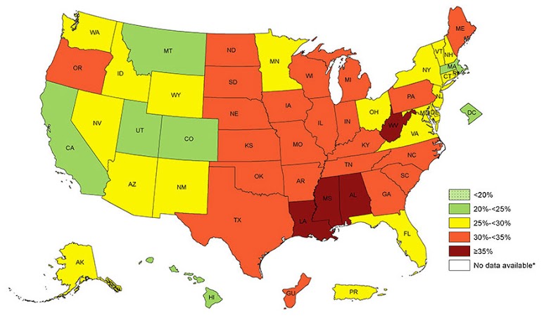 Prevalence of Self-Reported Obesity Among U.S. Adults by State and Territory, Behavioral Risk Factor Surveillance System, 2015.
Source: https://www.cdc.gov/obesity/data/prevalence-maps.html.
If the researcher further performs an analysis of these data in order to identify independent predictors of the health outcome, he or she must account for the spatial autocorrelation. Failure to do so may lead to biased estimates or incorrect conclusions about statistical significance. In this sense, the spatial autocorrelation is a nuisance that must be filtered out in the regression model. On the other hand, perhaps the health patterns and geographical variation is the predictor of interest. There are a variety of solutions to this problem, each with varying degrees of success, such as frequentist or Bayesian conditional autoregressive models, but one of the more straightforward and flexible solutions I've worked with is eigenvector spatial filtering. Its most attractive feature is it allows the use of typical regression techniques (i.e. generalized linear models with varying probability distributions) that many epidemiologists are well familiar with, and is applicable to multilevel modeling. Here's several articles I've found particularly helpful:
- Griffith DA, Peres-Neto PR. Spatial modeling in ecology: the flexibility of eigenfunction spatial analyses. Ecology. 2006 Oct;87(10):2603-13.
- Griffith DA. A comparison of six analytical disease mapping techniques as applied to West Nile Virus in the coterminous United States. Int J Health Geogr. 2005 Aug 2;4:18.
- Park YM, Kim Y. A spatially filtered multilevel model to account for spatial dependency: application to self-rated health status in South Korea. Int J Health Geogr. 2014 Feb 27;13:6.
Eigenvectors are a series of map patterns describing the spatial dependencies of the data. By their very nature, they are expected to account for the spatial autocorrelation and are distinct from one another (no multicollinearity). Users of R can turn to the SpatialFiltering function in the spdep package for generating what is known as the simultaneous autoregressive (SAR) spatial process. This function returns the optimally computed set of n eigenvectors, and these n eigenvectors are the ones the research is concerned with. Once computed, the researcher can utilize them in various ways. They can be plotted on a map to visualize areas with strong or weak autocorrelation. They can be described quantitatively. And they can be fitted into a GLM as fixed effects to control for the autocorrelation. When fitting as a covariate, the researcher can assess the amount of variability in the model explained by spatial autocorrelation (before and after R-squared), improved model fit (before and after AIC), and using Moran's I, ensure that spatial autocorrelation has been statistically accounted for in the model.
To actually carry out this analysis, the researcher needs to have a spatial dataset available in a shapefile specification as well as a neighbor matrix defined. See my previous blog post for an example of generating your own spatial files and neighbor matrix. To generate the matrix of selected eigenvectors via the SpatialFiltering function, the user specifies the spatial model to be fit in R formula syntax. For example,
spatial_eigen = SpatialFiltering(Outcome ~ 1, ~ Predictor - 1, data=dataset@data, nb=neighborhood_matrix, style="W", ExactEV=T)
We can then access the eigenvectors by calling fitted(spatial_eigen), where each column corresponds to an eigenvector (the number of columns is the number of eigenvectors selected). Each row is the specific eigenvalue for that spatial unit. To connect the eigenvalue with the appropriate spatial unit, one can iterate over the dataset and connect the row in the fitted(spatial_eigen) object that corresponds to the given spatial unit. There will be n number of new variables created for each observation, where n corresponds to the number of eigenvectors selected. For example, if ncol(fitted(spatial_eigen)) returns the value of 4, we need to add four eigenvalue variables to the dataset. For each spatial unit, we add the corresponding four eigenvalues. Finally, the eigenvalue variables are simply added as covariates to the regression model. If the spatial autocorrelation has been successfully accounted for, Moran's I statistic should be close to zero. Voila!
Cite: Goldstein ND. A straightforward solution to autocorrelation in epidemiology: eigenvector spatial analysis. Jul 14, 2017. DOI: 10.17918/goldsteinepi.