Assessing exposure in retrospective cohorts
A cohort is usually formed in an epidemiological study to assess the relationship of an antecedent exposure to an incident outcome. Ideally ensured in the study's design is the notion of temporality; exposure preceding the outcome offers greater evidence of causality. In a prospective cohort, ensuring temporality is easier (let's ignore outcomes with long incubation or latent periods). By its very nature the cohort is formed on the basis of an exposure, without knowledge of the eventual outcome (although there may be a suspicion as the basis of the hypothesis). In a retrospective cohort, ensuring temporality becomes more of a challenge. Not because the exposure has not preceded the outcome, but because more care needs to be given when operationalizing the exposure. This blog post serves as a caveat for those conducting a retrospective cohort.
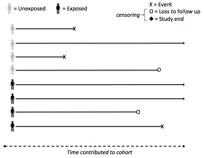
Take the above hypothetical cohort as an example. In a prospective study, the cohort is recruited on the basis of the exposure, hopefully ensuring some degree of temporality. In a retrospective study, we already have knowledge of the outcome. How do we operationalize the exposure ensuring temporality, and that the "at risk" period for each individual is correctly analyzed?
To make this more concrete, assume a cohort is formed to assess new cases of healthcare acquired infections in a hospital and the exposure is the average number of occupied beds during the patient's length of stay (perhaps mean or median dichotomized so it can be assessed as an exposure/unexposed predictor). We hypothesize that a higher average number of occupied beds will confer a greater risk for infection. The outcome is straightforward to operationalize: people will either have a diagnosed infection (outcome) or not (right censored). At first blush, the exposure can be operationalized by simply counting the number of occupied beds for each person's length of stay, and taking the average, repeated for each person in the cohort.
But wait: the exposure must precede the outcome. How do we do this? By defining the "at risk" period for each person in the cohort. For those that do not experience the outcome (the censored observations), the "at risk" period is truly the entire length of stay (again ignoring the incubation time of the pathogen). But for those that have the outcome, the "at risk" period is not the entire length of stay, but just the duration until they were diagnosed with the outcome. This should make intuitive sense, as this is exactly what we do in a prospective study. People stop contributing cohort time when they either experience the outcome or are censored. Thus as we operationalize the exposure, we must keep in mind that it is contingent upon the outcome. This is very different from a prospective cohort where we do not know the outcome at the outset.
Failure to consider the outcome will result in an information bias -- more specifically -- a differential misclassification of the exposure. That is, we incorrectly classified the exposure variable on the basis of the outcome. Unfortunately differential misclassification is difficult to predict which way this will bias the analysis. Not only do we need to calculate the exposure with this caveat in mind, but any covariate in the analysis where the "at risk" period may change during the cohort.
One way to do this is in the data management and recoding portion of the analysis. We can use an if-then-else statement to check the status of the outcome any time one of these "at risk" period covariates is created. Another easier way is to have a single if-then-else statement at the beginning of the recodes that captures the end date of the "at risk" period, thereby avoiding the continual checking of the outcome. The figure below is some pseudo code to accomplish this.
Cohort_start = Date_of_inception
Cohort_end = if (Outcome==True) then Date_of_outcome else if (Outcome==False) then Date_of_censor
At_risk_period = Cohort_end - Cohort_start
Now, when analyzing the cohort we have more accurately captured the exposure risk profile versus an outcome-agnostic classification.
Edit Mar 15, 2021: A lot of time has gone by since I created this post, but recently, as exemplified with several observational cohort studies of drug therapies during COVID-19, I was reminded of another issue that I did not discuss when operationalizing cohort time in a retrospective study: that of immortal person time. In this blog post, I already discussed the notion of calculating follow-up time in a retrospective cohort, and the potential for misclassification should one include person-time following the outcome. When operationalizing the exposure, one must equally guard against incorporating person-time prior to the exposure. This is known as immortal person time as although this individual may ultimately receive the exposure (at a later point in time) they are not at risk of the outcome prior to exposure. After all, one cannot receive the exposure if they have experienced the outcome already. While this seemingly minor detail may be appear obvious, it is not always so in the confines of the cohort. This often due to the sometimes ambiguous notion of the start period in a cohort study, which, unlike a randomized controlled trial with a very explicit start date, retrospective studies likely do not have such a clear definition.
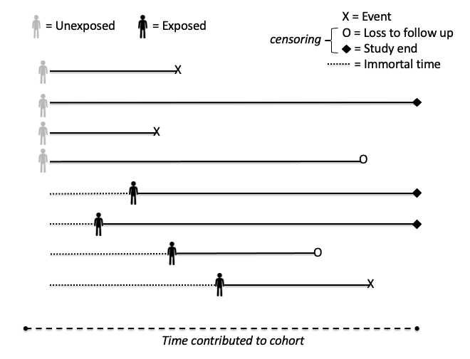
For example, consider the figure above. This retrospective cohort may have been operationalized based upon the admission date to the hospital (i.e., admission date is used as the date of cohort inception). The hypothetical exposure, suppose a medication, may not start at the date the cohort was assembled, especially if the medication relied upon a diagnosis that wasn't available at or immediately after admission. Analyzing the period of time prior to exposure as exposed results in a misclassification of person-time. If this misclassification is dependent upon the patient's outcome, then it becomes differential. On the other hand, discarding this information altogether (i.e., starting the cohort follow-up time clock ticking upon exposure) also has the potential to misclassify this individual. This type of information bias is more specifically known as immortal time bias. There are several ways to remediate this issue. One can consider a window of time to define the exposed group, say within 48 hours of hospital admission. In this case, even those exposed at a later point in time are still analyzed as unexposed. This is easy to implement and analyze, but unfortunately now those unexposed may be misclassified if they receive treatment later in their hospitalization. The best solution is where exposure is time-varying: that is, for each day, one creates an exposed (yes/no) variable that can be appropriately considered in analysis.
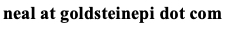
Cite: Goldstein ND. Assessing exposure in retrospective cohorts. Dec 23, 2015. DOI: 10.17918/goldsteinepi.