A simple presentation of error rates, effect size, and sample
In the introductory epidemiology class I teach, I've had this question posed to me several times: "Can you define the relationship between the error types and sample size?" Of course there is a relationship between these, as well as the effect size, as those components are the required parameters in most sample size equations.
Lowering alpha or beta - and thus lowering risk of type I or II error rates - means you are asking for greater confidence in your answer. Requesting greater confidence (i.e., increasing precision) in your answer translates to more data points, which often means more people (or more measurements of those people). For example, going from an standard alpha of 0.05 to an alpha of 0.01 will increase sample size as will going from a beta of 0.20 (80% power) to a beta of 0.10 (90% power). Likewise, a weaker effect will also demand a larger sample.
I was planning to refer the student to previously published power and sample size curves, but having had difficulty finding them I decided to create a few graphs depicting this relationship. This blog post serves as a way to share these graphs with others who may find this beneficial as well as share the R code I used to create these graphs. These were created by performing a sample size calculation for Pearson correlations of two continuous variables across a range of effect sizes, alphas, and betas. Notes on each figure depict assumptions. All were calculated as two-sided hypotheses. If you do find these useful, please cite this resources. Thanks and enjoy!
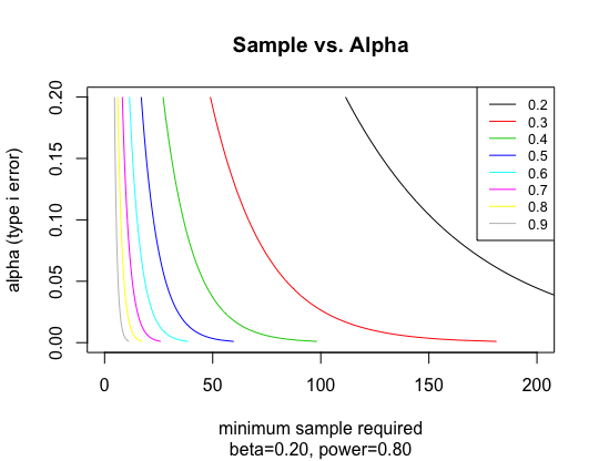
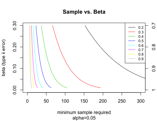
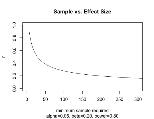
################# # Sample size curves # Requires:# 11/6/18 -- Neal Goldstein ################# ### FUNCTIONS ### library(pwr) ### ALPHA (TYPE I ERROR) ### #range of correlation coefficients r = seq(0.2,0.9,0.1) #range of alpha values alpha = seq(0.001,0.20,0.001) #initialize plot plot(NULL, xlim=c(0,200), ylim=c(0,0.2), xlab="minimum sample required", ylab="alpha (type i error)", main="Sample vs. Alpha", sub="beta=0.20, power=0.80") #calculate sample size over all correlations and alpha values for (j in 1:length(r)) { sample_alpha = NA for (i in 1:length(alpha)) { sample_alpha = c(sample_alpha, pwr.r.test(n=NULL, r=r[j], sig.level=alpha[i], power=0.8, alternative="two.sided")$n) } sample_alpha = sample_alpha[-1] #add sample size curves to plot lines(sample_alpha, alpha,col=palette()[j]) } #add legend legend("topright",legend=r, lty=rep(1,8),col=palette(), cex=0.8) ### BETA (TYPE II ERROR) ### #range of correlation coefficients r = seq(0.2,0.9,0.1) #range of beta values beta = seq(0.01,0.30,0.001) #initialize plot plot(NULL, xlim=c(0,300), ylim=c(0,0.3), xlab="minimum sample required", ylab="beta (type ii error)", main="Sample vs. Beta", sub="alpha=0.05") axis(4, at=c(0,0.10,0.20,0.30), labels=(1-c(0,0.10,0.20,0.30))) #calculate sample size over all correlations and alpha beta for (j in 1:length(r)) { sample_beta = NA for (i in 1:length(beta)) { sample_beta = c(sample_beta, pwr.r.test(n=NULL, r=r[j], sig.level=0.05, power=(1-beta[i]), alternative="two.sided")$n) } sample_beta = sample_beta[-1] #add sample size curves to plot lines(sample_beta, beta,col=palette()[j]) } #add legend legend("topright",legend=r, lty=rep(1,8),col=palette(), cex=0.8) ### EFFECT SIZE ### #range of correlation coefficients r = seq(0.1,0.9,0.01) #initialize plot plot(NULL, xlim=c(0,300), ylim=c(0,1), xlab="minimum sample required", ylab="r", main="Sample vs. Effect Size", sub="alpha=0.05, beta=0.20, power=0.80") #calculate sample size over all correlations sample_r = NA for (j in 1:length(r)) { sample_r = c(sample_r, pwr.r.test(n=NULL, r=r[j], sig.level=0.05, power=0.80, alternative="two.sided")$n) } sample_r = sample_r[-1] #add sample size curves to plot lines(sample_r, r)
Cite: Goldstein ND. A simple presentation of error rates, effect size, and sample. Nov 6, 2018. DOI: 10.17918/goldsteinepi.